PyGamma is a fantastic python library that provides a wrapper around the C++ library Gamma (General Approach to Magnetic resonance Mathematical Analysis). Simulating NMR or MRS spectra with PyGamma is easy, however, the examples that come bundled with PyGamma a little limited if you just want a quick simulation. So let us have a look at a modified version of the example FID pulse sequence in PyGamma to get our acquisition table mx (if you just want the code without the explanation, you can go here).
GABA simulation
Setup
First, lets set up a python virtual environment to run this, based on the requirements found with the code here. A range of systems are included under ‘sys/’, generally, these systems have the Govindaraju et al. values. There’s a range of 23 of metabolites in there, including NAA, Creatine, Glutamine, Glutamate, I’d double check these if you need specific or exact values.
virtualenv venv && source venv/bin/activate && pip install -r requirements.txt
import pygamma as pg

def fid(sys, b0=123.23):
    sys.OmegaAdjust(b0)
    H = pg.Hcs(sys) + pg.HJ(sys)
    D = pg.Fm(sys)
    ACQ = pg.acquire1D(pg.gen_op(D), H, 0.1)
    sigma = pg.sigma_eq(sys)
    sigma0 = pg.Ixpuls(sys, sigma, 90.0)
    mx = pg.TTable1D(ACQ.table(sigma0))
    return mx
This is a modified version of the example fid.py that can be found here. There’s a couple of additional parts added here, first we’ve wrapped the ACQ.table in a pg.TTable1D() to stop the C table object being garbage collected when we exit the fid function. This means we can pass the mx table object around between methods. Secondly, I’ve added the ability to adjust the b0 frequency (in MHz) of the scanner via Omega adjust.
Next, we need to take the mx object and get it to return our FID, FFT and nu. If you’re interested in the methods invoked here, check out the L2 section of the Gamma user guide here.
def binning(mx, b0=123.23, high_ppm=-3.5, low_ppm=-1.5, dt=5e-4, npts=4096, linewidth=1):
    mx.broaden(linewidth)       # add some broadening
    mx.resolution(0.5)          # Combine transitions within 0.5 rad/sec

    ADC = []
    acq = mx.T(npts, dt)
    for ii in range(0, acq.pts()):
        ADC.extend([acq.get(ii).real() + (1j * acq.get(ii).imag())])

    FFT = []
    acq = mx.F(npts, b0 * high_ppm, b0 * low_ppm)
    for ii in range(0, acq.pts()):
        FFT.extend([acq.get(ii).real() + (1j * acq.get(ii).imag())])

    ADC = normalise_complex_signal(np.array(ADC))
    FFT = normalise_complex_signal(np.array(FFT))
    nu = np.linspace(high_ppm, low_ppm, npts)

    return ADC, FFT, nu
The FFT returned by PyGamma is not the same as FFT(ADC), rather than having a bandwidth determined by acquisition parameters, it has the exact frequency range specified by low_ppm and high_ppm. There’s also small function included for normalizing the complex signals to be within the range [-1:1]. This makes plotting our data much nicer:
def normalise_complex_signal(signal):
    return signal / np.max([np.abs(np.real(signal)), np.abs(np.imag(signal))])
Finally, let’s build some plots for this data.
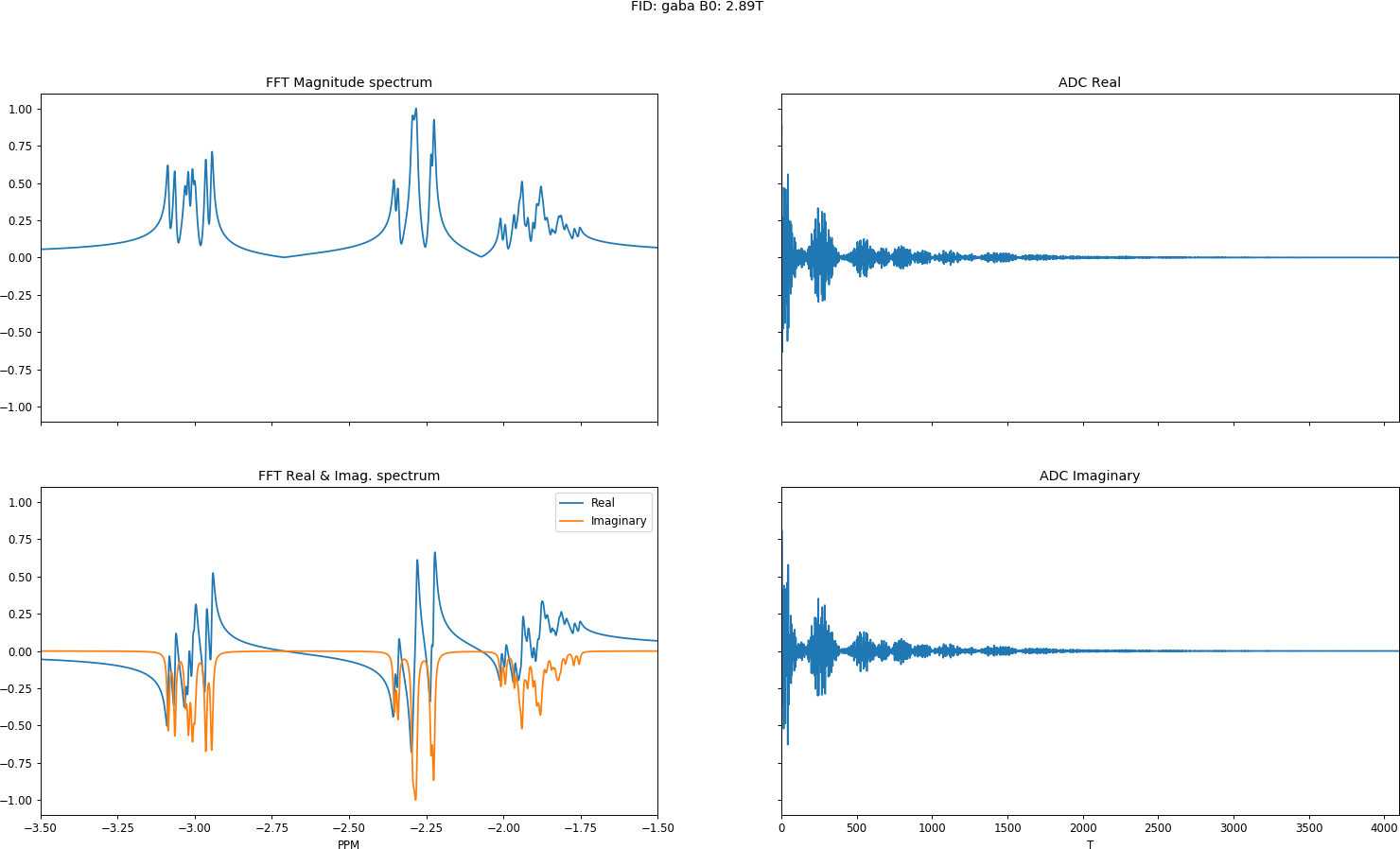
def plot(sys, ADC, FFT, nu):
    fig, axes = plt.subplots(2, 2, sharex='col', sharey=True,  figsize=(19.2, 10.8), dpi=85)
    # pulse sequence name, system name and magnetic field strength
    plt.suptitle('FID: %s B0: %.2fT' %(sys.name(), hz_to_tesla(sys.Omega())))

    # Plot the reported FFT from PyGamma
    axes[0, 0].set_title('FFT Magnitude spectrum')
    axes[0, 0].plot(nu, np.abs(FFT)/max(np.abs(FFT)))
    axes[0, 0].set_xlim([min(nu), max(nu)])

    axes[1, 0].set_title('FFT Real & Imag. spectrum')
    axes[1, 0].plot(nu, np.real(FFT), label='Real')
    axes[1, 0].plot(nu, np.imag(FFT), label='Imag')
    axes[1, 0].set_xlabel('PPM')
    axes[1, 0].legend(['Real', 'Imaginary'])

    # Plot the ADC
    axes[0, 1].set_title('ADC Real')
    axes[0, 1].plot(np.linspace(0, len(ADC), len(ADC)), np.real(ADC))
    axes[0, 1].set_xlim([0, len(ADC)])

    axes[1, 1].set_title('ADC Imaginary')
    axes[1, 1].plot(np.linspace(0, len(ADC), len(ADC)),np.imag(ADC))
    axes[1, 1].set_xlabel('T')

    plt.show()
Loading, simulation and binning for GABA a 6 spin system takes 0.03 seconds on my dual-core laptop.
Code for this and all my PyGamma examples can be found on GitHub.